Compression Is Intelligence: A Mathematical Argument, and Its Limits

For most of the last century, intelligence was treated as a philosophical or biological category — a quality you recognized by its effects (insight, wit, understanding) but could not pin to an equation. Algorithmic Information Theory (AIT) offers a startling alternative: intelligence, in the fullest sense we can currently formalize, is nothing more than the ability to compress data optimally. Predicting the future and compressing the past turn out to be the same mathematical operation viewed from two angles. This essay builds that argument from first principles — through Shannon's entropy, Kolmogorov complexity, Solomonoff induction, and Hutter's AIXI — traces its concrete embodiment in how large language models are trained, and then examines where the equivalence strains, and what it leaves out.

1. Shannon's Limit: Why Compression Has a Floor

Claude Shannon's 1948 paper A Mathematical Theory of Communication began from a narrow engineering problem — how many bits does a message really need? — and ended up defining the unit of "surprise" itself.

Fixed-width encodings like ASCII are wasteful because they spend the same eight bits on a common letter like "e" and a rare symbol like ";". An optimal code instead assigns short bitstrings to frequent events and long ones to rare events, in exact inverse proportion to their probability. For this scheme to be decodable without delimiters, it must be prefix-free: no valid code word can be the prefix of another. The Kraft–McMillan inequality formalizes the tradeoff this creates — every short codeword you hand out consumes a disproportionate share of the space of possible codes, so an optimal encoding must saturate that space with no waste left over.

Push this idea to its limit and something interesting happens: a perfectly compressed message contains no further exploitable pattern, because any remaining pattern would itself be compressible. So maximal compression converges toward statistical randomness — not because the underlying message was random, but because every regularity has already been extracted and reused. This gives us a precise definition of information content. If a sequence of length $n$ is drawn from a source where every outcome is equally likely, each specific outcome has probability $p = 2^{-n}$, and solving for bit-length gives:

$$I = -\log_2(p)$$

Rare events carry more bits of "surprise" than common ones — a formal version of the everyday intuition that news is only news when it's unexpected. Averaging this surprise across an entire distribution gives entropy:

$$H = -\sum_{i} p_i \log_2(p_i)$$

Entropy is the theoretical floor beneath which no lossless compressor can go, for a source that truly matches that distribution. It is worth being precise about what this floor depends on: it is fixed only relative to a known, stationary probability distribution. Real data — language, images, planetary orbits — doesn't announce its distribution in advance. Finding that distribution is the actual work, and it's here that the story stops being pure information theory and starts becoming a theory of intelligence.

2. From Statistics to Algorithms: Kolmogorov Complexity

Shannon entropy measures uncertainty relative to a given probability model. But where does the model come from? A purely statistical compressor — one that just counts symbol frequencies — will do a mediocre job on something like a table of planetary positions. It might shave off some redundancy by noting which digits repeat, but it will never approach the real compressibility of the data, because the real compressibility isn't statistical at all. It's causal: the positions were generated by Newtonian gravity, $F = Gm_1m_2/r^2$, and a few bytes of formula plus initial conditions reproduce gigabytes of coordinates exactly.

This is the insight formalized by Andrey Kolmogorov and, independently, Ray Solomonoff and Gregory Chaitin. The Kolmogorov complexity $K(x)$ of a string $x$ is the length of the shortest program that, run on a fixed universal computer $U$, outputs $x$ and halts:

$$K(x) = \min_{p} {\, |p| : U(p) = x \,}$$

This reframes compression as program search rather than frequency counting, and it reframes scientific discovery as a special case of compression: a physical law is a short program for a long dataset. It also comes with an honest, load-bearing caveat that popular treatments of this idea often omit: $K(x)$ is not computable. There is no algorithm that takes an arbitrary string and returns its true Kolmogorov complexity, because doing so would require solving the halting problem — you can never be certain a shorter generating program doesn't exist somewhere in the infinite space of programs you haven't checked. Kolmogorov complexity is therefore a theoretical ideal, not a metric you can compute in practice. Every real compressor — gzip, a neural network, a human scientist — is a bounded approximation reaching for this uncomputable target. That gap between the ideal and the achievable is not a footnote; it's the entire reason machine learning research exists as an empirical field rather than a solved theorem.

3. Occam's Razor, Made Rigorous: Solomonoff Induction

If perfect compression requires an uncomputable oracle, how should a real reasoner allocate its belief across competing explanations of the data it has seen? Ray Solomonoff answered this in 1960 with a formal theory of induction that mathematically justifies Occam's razor — the idea that, among hypotheses fitting the evidence equally well, we should favor the simplest.

Solomonoff's universal prior assigns each hypothesis a probability derived from the length of the programs that produce it:

$$P(x) = \sum_{p \,:\, U(p) = x} 2^{-|p|}$$

Because $2^{-|p|}$ shrinks exponentially with program length, short programs dominate this sum — simplicity isn't a tie-breaking aesthetic preference here, it's the mathematically inevitable consequence of weighting hypotheses by their description length. Combined with Bayes' rule, this gives an idealized inductive agent whose cumulative prediction errors are provably bounded by the Kolmogorov complexity of whatever process is actually generating the data. An agent that compresses optimally predicts optimally, and vice versa — the two are not merely correlated but formally identical.

Like $K(x)$, Solomonoff induction is uncomputable. It requires summing over every program that could produce the observed data, including infinitely many that never halt. It is the "AIXI of prediction" in the sense that it defines a ceiling nothing can reach exactly — but, as with physical limits like the speed of light, defining the ceiling tells you which direction progress lies in.

4. AIXI: From Prediction to Universal Agency

Solomonoff's theory handles pure prediction — what comes next? — but intelligence in the everyday sense also involves acting to achieve goals under uncertainty. Marcus Hutter's AIXI, introduced around 2000, closes this gap by fusing Solomonoff induction with reinforcement learning: an AIXI agent picks the action, at every timestep, that maximizes expected future reward under a Solomonoff-weighted distribution over all computable environments consistent with its history so far.

This produces a genuinely general definition of intelligence — Hutter and Shane Legg later formalized it as an agent's expected performance across the full space of computable reward-generating environments, weighted by simplicity. It also inherits every practical limitation of its ingredients: it is uncomputable, it assumes a stationary and fully specifiable reward signal, and it says nothing about how to build a tractable approximation, only what the target looks like. Hutter's own response to that gap is instructive: rather than leave the idea purely theoretical, he founded the Hutter Prize for compressing a large snapshot of Wikipedia as densely as possible, on the reasoning that squeezing human-written text losslessly forces an algorithm to internalize grammar, facts, and world structure — compression as an empirical proxy for the uncomputable ideal.

5. Cross-Entropy: How Compression Becomes a Training Signal

Everything so far has been about defining an ideal. Cross-entropy is the bridge that turns the ideal into something you can actually optimize with gradient descent.

If reality generates outcomes according to a true distribution $P$, and a model navigates the world with an internal, possibly wrong distribution $Q$, then the expected number of bits needed to encode reality's outcomes using the model's mistaken code is the cross-entropy:

$$H(P, Q) = -\sum_{i} P_i \log_2(Q_i)$$

This is provably minimized only when $Q = P$ — that is, when the model's beliefs exactly match reality — which is why it functions as a distance between "what the model thinks" and "what is actually true." The gap above the true floor is the Kullback–Leibler divergence:

$$D_{\text{KL}}(P \parallel Q) = H(P, Q) - H(P) = \sum_i P_i \log_2\!\left(\frac{P_i}{Q_i}\right)$$

Since a fixed dataset has fixed entropy $H(P)$, minimizing cross-entropy and minimizing KL divergence are the same optimization problem. This is precisely how a transformer is trained: at each position, it outputs a predicted distribution $Q$ over the next token, the dataset supplies the true (one-hot) distribution $P$, and the loss collapses to the negative log-likelihood of the correct token, $-\log(Q_\text{true})$. Training an LLM is, quite literally, running an approximate, computable, gradient-based search for a short program that compresses the entirety of its training corpus — the empirical, tractable cousin of the uncomputable Solomonoff search described above.

It is also worth noting why the loss must be logarithmic rather than some other penalty function, since this is often stated without justification: it can be shown via constrained optimization (Lagrange multipliers) that if you require a loss function whose minimum coincides exactly with the model matching the true data distribution — no more, no less — the logarithmic form is forced by the constraint, not chosen by convention. Cross-entropy isn't merely a convenient loss function that happens to work; it's the unique function satisfying that requirement.

6. Distillation and "Dark Knowledge"

Cross-entropy's role doesn't end at pretraining — it also explains how models teach other models. In knowledge distillation, a smaller "student" network is trained not on raw text but on the soft probability distribution output by a larger "teacher" model. Where the raw dataset offers a brutal one-hot signal (the correct word gets probability 1, everything else gets 0), the teacher's softened output over the vocabulary — high probability on "cat," moderate on "dog," near-zero on "democracy" — encodes relational structure between concepts that the one-hot target throws away entirely. Geoffrey Hinton called this residual signal "dark knowledge": information about how concepts relate to one another, invisible in the ground-truth label but present in the shape of the teacher's uncertainty. Because $H(P)$ for the dataset is fixed regardless of which model is doing the predicting, distillation is just another instance of KL minimization — the student compresses the teacher's model of the world rather than compressing the raw world directly, one level of indirection up the same stack.

7. Why Language Entropy Is Low, and What That Reveals

Early information theorists tested these ideas directly on people. In Shannon's own "guessing game" experiments, subjects predicted upcoming characters in English text with startling accuracy given sufficient context, and later refinements of this method converged on an estimate near one bit per character for English — dramatically below the ~4.7 bits per character implied by treating each of the 26-ish possible characters as equally likely. (Later corpus-based estimates using neural language models refine this somewhat, typically landing in the 1–1.3 bit range depending on genre and context length — Shannon's hand-estimate has held up remarkably well but was never meant as an exact constant.)

This gap between the naive and true entropy of language reveals two things at once. First, language is saturated with redundancy that functions as built-in error correction — you can drop letters, garble grammar, or hear a sentence over a bad phone line and still recover the meaning, because far more information is present than the theoretical minimum requires. Second, and more importantly, humans don't achieve this predictive accuracy by unconsciously computing character frequencies. They do it because they carry an internal causal model of the world. "The dropped glass shattered on the _" is easy to complete not from n-gram statistics but from an intuitive grasp of gravity, fragility, and the existence of floors. Low entropy in the output is the symptom; a rich generative model of reality is the cause.

This is the pivot point of the whole essay's argument: to drive a model's cross-entropy loss down toward that ~1-bit floor across the full breadth of human-generated text, a system cannot rely on surface statistics. The contexts are too varied, too long-range, and too dependent on facts about physics, social convention, mathematics, and causality. Achieving near-optimal compression forces the construction of an internal world model as a side effect of loss minimization — not because anyone programmed the model to reason, but because reasoning is cheaper, in bits, than memorizing every surface pattern separately. Empirical work by DeepMind ("Language Modeling Is Compression," 2023) made this concrete: general-purpose LLMs, run as arithmetic coders, out-compress specialized tools like PNG and FLAC on their respective data types, and compression ratio on held-out text correlates closely with downstream reasoning benchmark scores — evidence that the theoretical link between compression and capability shows up empirically, not just on paper.

8. Where the Equivalence Strains

The argument above is genuinely powerful, but treating "intelligence = compression" as a closed, settled identity glosses over real tension points worth naming honestly.

Compression is necessary but arguably not sufficient. A system can compress a corpus extremely well through sophisticated memorization and shallow pattern-matching without possessing anything most people would call understanding or agency — a large enough lookup table with enough interpolation can drive loss down substantially. The theoretical guarantee (Solomonoff's error bound) applies to an idealized, uncomputable predictor; nothing guarantees that a finite, gradient-trained approximation inherits that guarantee in full. This is precisely why the gap between "the loss went down" and "the model reasons" remains an active empirical and philosophical question rather than a corollary of the math.

Prediction is not the same as goal-directed action. AIXI patches this by wrapping Solomonoff induction in reinforcement learning, but that patch introduces its own unresolved questions — a stationary, fully specifiable reward signal is a strong and often unrealistic assumption, and "acts to maximize reward across all computable environments" is a different, broader claim than "predicts text well." Passive prediction and active, embodied, goal-pursuing intelligence are related but not identical phenomena, and collapsing them risks eliding the difference between a system that models the world and one that must also act in it under real consequences.

Lossy versus lossless matters. Much of this essay's argument (and the Hutter Prize) is framed around lossless compression, where nothing can be discarded and every irregularity must be accounted for. But human cognition, and most useful machine learning, is thoroughly lossy — we forget, generalize, and discard detail constantly, and that discarding is often what generalization is. The Minimum Description Length principle (a close statistical cousin of Kolmogorov complexity) formalizes this tradeoff explicitly: the best model is the one minimizing the combined cost of describing the model plus describing the data's exceptions under that model, which explicitly rewards forgetting irrelevant detail rather than penalizing it. A pure lossless-compression framing undersells how much of intelligence is selective forgetting, not exhaustive retention.

Uncomputability is a real ceiling, not a rhetorical flourish. Kolmogorov complexity, Solomonoff induction, and AIXI are all formally uncomputable. That doesn't make them useless — physics is full of idealizations (frictionless planes, point masses) that guide real engineering without ever being achieved exactly — but it does mean every real system, including the largest LLMs, is a bounded, heuristic approximation of an unreachable target, not an implementation of it. Claims that any specific model "is" doing Solomonoff induction should be read as "is a rough, resource-limited approximation of," which is a meaningfully weaker and more honest statement.

9. Synthesis

None of these caveats overturn the central thesis; they sharpen it. Shannon showed that compression has a hard mathematical floor set by entropy. Kolmogorov and Solomonoff showed that reaching that floor on complex, structured data requires discovering the generative process behind it, not just its surface statistics — though the ideal version of that discovery is provably uncomputable. Hutter showed how to fold that predictive ideal into a general theory of goal-directed agency, at the cost of inheriting the same uncomputability plus new assumptions about reward. Cross-entropy and KL divergence supply the actual, computable, differentiable proxy that lets real systems climb toward these ideals via gradient descent, and distillation shows the same compression logic operating one level removed, model-to-model rather than model-to-world. And the empirically low entropy of human language is the clue that ties it together: squeezing language down toward its true information floor is only possible by building something that behaves, functionally, like a model of the world it describes.

Intelligence, on this account, is not a separate ingredient added to prediction — it's what sufficiently good, sufficiently general prediction becomes once the data being predicted is rich enough that no shortcut around understanding remains cheaper than understanding itself. That is a genuine and defensible mathematical insight. It is just not, on its own, a complete theory of mind — and treating it as one, rather than as a rigorous lower bound with real open questions above it, is the essay's one avoidable overreach worth resisting.

10. Mathematical equivalence

The equivalence between intelligence and compression is formally grounded in Algorithmic Information Theory. The core mathematical idea is that the ability to understand, predict, and act intelligently is identical to finding the shortest possible program to describe a dataset (lossless compression).

Here are the most rigorous ways to express this succinctly:

1. The Universal Intelligence Measure

Proposed by Shane Legg and Marcus Hutter, this formula defines the intelligence of an artificial agent ($\Upsilon$) based on the Kolmogorov complexity ($K$) of the environments it can successfully navigate:

$$\Upsilon(\pi) = \sum_{\mu \in E} 2^{-K(\mu)} V_{\mu}^{\pi}$$

• $\Upsilon(\pi)$: The universal intelligence of agent $\pi$.

• $K(\mu)$: The Kolmogorov complexity (maximum compression/minimum description length) of environment $\mu$.

• $V_{\mu}^{\pi}$: The expected reward the agent achieves.

• $2^{-K(\mu)}$: The algorithmic probability factor, which weights highly compressible, simpler environments more heavily.

2. Solomonoff Induction (Prediction as Compression)

If intelligence is the ability to predict future data based on past observations, Ray Solomonoff proved the optimal predictor relies entirely on finding the most compressed representation:

$$P(x) = \sum_{U(p)=x} 2^{-\vert{}p\vert{}}$$

• $P(x)$: The probability of a data sequence $x$.

• $\vert{}p\vert{}$: The length in bits of program $p$ running on a Universal Turing Machine $U$ that outputs $x$.

• This demonstrates that the shortest programs (the best compression) mathematically dominate the probability of what happens next.

3. The Conceptual Shorthand

We express that intelligence ($I$) is inversely proportional to the minimal description length or Kolmogorov complexity ($K$) of a given dataset ($D$):

$$I \propto \frac{1}{K(D)}$$

4. The Calculus of Surprise — Where Perplexity Meets Compression

To bridge the abstract realm of Algorithmic Information Theory (Kolmogorov complexity) with the practical reality of modern artificial intelligence, we must introduce the metric that actually drives machine learning: Perplexity.

If Kolmogorov complexity $K(D)$ represents the absolute, theoretical limit of compression, perplexity represents how close a real-world predictive model is getting to that limit. In the context of intelligence, perplexity is the mathematical measure of surprise.

1. Defining Perplexity Conceptually

When an intelligent agent observes a sequence of events (or words in a sentence, or moves in a chess game), it constantly builds a probability distribution of what will happen next.

• If the agent deeply understands the underlying rules of the environment, it will assign a high probability to the actual next event. It is not surprised.

• If the agent lacks understanding, it will assign equal probability to many possible random outcomes. When the actual event occurs, the agent is highly surprised.

Perplexity quantifies this surprise. A low perplexity means the model's predictions tightly match reality (high understanding). A high perplexity means the model is essentially guessing uniformly at random (low understanding).

2. The Mathematical Bridge: Entropy and Bits

To see how perplexity is strictly identical to compression, we must route it through Shannon Entropy ($H$).

In information theory, the entropy of a sequence of data $X$ given a model's predicted probability distribution $q(x)$ is the average number of bits required to encode (compress) each piece of data. This is known as cross-entropy:

$$H = -\frac{1}{N} \sum_{i=1}^{N} \log_2 q(x_i)$$

Here, $N$ is the number of tokens/events, and $q(x_i)$ is the probability the model assigned to the correct event $x_i$. The better the model understands the data, the higher $q(x_i)$ is, and the smaller the cross-entropy $H$ becomes.

Perplexity ($PP$) is simply the exponentiation of this entropy:

$$PP = 2^H$$

If a model requires an average of $3$ bits to compress each word in a document, its perplexity is $2^3 = 8$. This means that, mathematically, the model is as confused as if it had to choose uniformly between $8$ equally likely options at every step.

3. The Equivalence: Minimizing Surprise is Maximizing Compression

We can now cleanly align perplexity with our previous shorthand for intelligence, $I \propto \frac{1}{K(D)}$.

Modern Large Language Models (LLMs) do not directly calculate Kolmogorov complexity, because $K(D)$ is technically uncomputable—you can never definitively prove you have found the absolute shortest possible program. Instead, they minimize cross-entropy loss, which directly minimizes perplexity.

By lowering perplexity, the model is quite literally reducing the number of bits required to store the dataset.

• High Perplexity: The model needs many bits per token. The resulting compressed file is large.

• Low Perplexity: The model needs very few bits per token. The resulting compressed file is tiny.

If we let $L$ represent the total compressed description length of a dataset of size $N$ achieved by a specific model, then $L = N \cdot H$. Substituting this back into the perplexity equation gives:

$$PP = 2^{\frac{L}{N}}$$

4. Intelligence as a Byproduct

This equation demonstrates that driving perplexity down is mathematically synonymous with driving the description length $L$ down toward the theoretical limit $K(D)$.

To minimize perplexity across a vast, complex dataset like the entirety of the human internet, an algorithm cannot rely on memorization (which would require too many bits). It is forced to develop internal representations of syntax, logic, physics, coding structures, and reasoning.

Therefore, intelligence is not programmed; it is the forced byproduct of an algorithm relentlessly optimizing to compress data by minimizing its own perplexity.

N-Body Simulator: A Deep Dive into Interactive Gravitational Physics

This document details an N-Body simulator, a program designed to visually and interactively demonstrate gravitational interactions between multiple bodies. The core functionality revolves around solving the N-Body problem, a classic challenge in physics concerning the prediction of motion for a system of celestial objects governed solely by Newtonian gravity. The simulator prioritizes accuracy, user interaction, and educational value, allowing users to explore complex gravitational scenarios with relative ease.

The simulator’s foundation lies in the numerical solution of Newton’s Law of Universal Gravitation and Newton’s Second Law of Motion. Instead of attempting analytical solutions (which are only possible for the two-body problem), the simulator employs a time-stepping method. This involves discretizing time into small intervals and calculating the gravitational force on each body at each time step. This force is then used to update the body’s velocity and position, effectively simulating its trajectory. The accuracy of the simulation is directly tied to the size of the time step; smaller time steps yield more accurate results but require greater computational resources.

Several integration methods are implemented to enhance accuracy and stability. The primary method is the Verlet integration scheme, known for its good energy conservation properties, crucial for long-term simulations. Verlet integration is symplectic, meaning it preserves the fundamental structure of Hamiltonian systems, minimizing energy drift over extended periods. However, the simulator also offers alternative integration methods, including the Euler method (simpler but less accurate, prone to energy drift) and the Runge-Kutta 4th order method (RK4, more accurate than Euler but computationally more expensive than Verlet). Users can select the integration method based on their desired balance between accuracy and performance.

The simulator allows for a high degree of user control over the simulation parameters. Users can define the number of bodies (N), ranging from two to potentially hundreds, although performance degrades with increasing N. For each body, users can specify initial position (x, y coordinates), initial velocity (vx, vy components), and mass. The gravitational constant (G) is also adjustable, allowing exploration of different gravitational strengths. Furthermore, users can modify the time step size, the integration method, and the simulation duration.

A key feature is the interactive nature of the simulation. Users can pause, resume, and reset the simulation at any time. They can also interact with individual bodies during a paused simulation, modifying their properties (position, velocity, mass) to observe the immediate effects on the system. This interactive capability is particularly valuable for educational purposes, allowing users to experiment with different scenarios and gain a deeper understanding of gravitational dynamics.

The visual representation of the simulation is designed for clarity and information density. Bodies are represented as points or small circles, with their size optionally scaled to reflect their mass. The simulation displays the trajectories of the bodies as lines, providing a visual record of their paths. A real-time display of simulation parameters, such as the current time, time step size, and total energy of the system, is also provided. The simulator includes options for adjusting the scale of the display, zooming in and out to focus on specific regions of the simulation. Color-coding of bodies is implemented to aid in distinguishing them, especially in simulations with a large number of bodies.

The simulator includes pre-defined scenarios to demonstrate various gravitational phenomena. These include:

• Two-Body Problem: Demonstrates stable orbits, elliptical paths, and the effects of varying masses and initial velocities.

• Three-Body Problem (Figure-Eight Solution): Illustrates a classic chaotic solution to the three-body problem, where three bodies of equal mass trace a figure-eight pattern.

• Alpha Centauri System: A simplified model of the Alpha Centauri star system, showcasing the gravitational interactions between multiple stars.

• Solar System Model: A scaled-down representation of our solar system, demonstrating the orbits of planets around the sun.

• Custom Scenarios: Users can create and save their own custom scenarios, allowing for exploration of arbitrary configurations of bodies.

Beyond the core simulation functionality, the simulator incorporates features for data logging and analysis. The simulator can record the position, velocity, and energy of each body at each time step, allowing users to export this data for further analysis using external tools. This capability is useful for investigating long-term trends, calculating orbital parameters, and verifying the accuracy of the simulation. The simulator also provides basic plotting capabilities, allowing users to visualize the trajectories of bodies and the evolution of energy over time.

The simulator’s development prioritizes performance optimization. The core simulation logic is implemented in a computationally efficient manner, leveraging optimized numerical algorithms and data structures. The visual rendering is also optimized to minimize overhead, allowing for smooth and responsive simulations even with a large number of bodies. The simulator is designed to be cross-platform, running on a variety of operating systems.

Future development plans include:

• Collision Detection: Implementing collision detection between bodies, allowing for realistic simulations of impacts and mergers.

• Relativistic Effects: Incorporating relativistic corrections to Newton’s Law of Gravitation, enabling simulations of strong gravitational fields.

• Advanced Visualization: Adding more sophisticated visualization options, such as 3D rendering and particle effects.

• User Interface Improvements: Enhancing the user interface to make the simulator more intuitive and user-friendly.

• Multi-threading: Utilizing multi-threading to further improve performance, especially for simulations with a large number of bodies.

In conclusion, the N-Body simulator is a powerful and versatile tool for exploring gravitational physics. Its combination of accuracy, interactivity, and educational features makes it valuable for students, researchers, and anyone interested in understanding the dynamics of celestial systems.

This article by Max Slater explores the powerful concept of representing functions as infinite-dimensional vectors, which allows the tools of linear algebra to be applied to problems in computer graphics, signal processing, and machine learning. The central thesis is that by formalizing this analogy, complex operations on functions can be simplified through techniques like diagonalization.

Functions as Infinite-Dimensional Vectors

The foundation of this concept lies in reinterpreting what a vector is. A standard N-dimensional vector can be seen as a map from a finite set of indices (e.g., {1, 2, ..., N}) to a set of values. By extending this idea, a function defined on the natural numbers, like a sequence, can be viewed as a vector with countably infinite dimensions. The crucial leap is to consider functions defined on the real numbers, which correspond to vectors with an uncountably infinite number of dimensions, where each real number serves as an index. This perspective, rigorously defined in functional analysis, allows for a powerful intuitive bridge from finite-dimensional linear algebra.

Formalizing the Analogy: Vector Spaces and Linear Operators

To treat functions as vectors formally, they must be shown to form a vector space. For the set of real-valued functions, this is achieved by defining vector addition and scalar multiplication in a pointwise manner:

• Vector Addition: (f + g)[x] = f[x] + g[x]

• Scalar Multiplication: (αf)[x] = αf[x]The zero vector is the function that is zero everywhere. These definitions satisfy all the necessary vector space axioms (commutativity, associativity, etc.), confirming that functions can indeed be treated as vectors.

Just as matrices are linear transformations on finite vectors, linear operators are linear transformations on functions. A prime example is the differentiation operator, d/dx, which is linear because the derivative of a linear combination is the linear combination of the derivatives. By considering a specific basis, such as the power basis (1, x, x², ...) for the space of polynomials, differentiation can be represented as an infinite-dimensional matrix that transforms the vector of a polynomial's coefficients.

Diagonalization and Eigenfunctions

A core technique in linear algebra is diagonalization, where a matrix A is decomposed into UΛU⁻¹. The columns of U are the eigenvectors of A—vectors that are only scaled by the transformation (Av = λv). The diagonal matrix Λ contains the corresponding scaling factors, or eigenvalues.

This concept extends to functions, where an eigenfunction of a linear operator L is a function f such that Lf = ψf, where ψ is the eigenvalue. The article attempts to diagonalize the differentiation operator by finding its eigenfunctions. Solving the differential equation df/dx = ψf yields exponential functions of the form Ce^(ψx). However, the differentiation operator cannot be fully diagonalized in the space of real functions because its eigenfunctions (real exponentials) do not form a basis capable of representing all analytic functions (e.g., polynomials like f[x] = x).

Inner Products and the Spectral Theorem

To find a more useful diagonalization, the concept of an inner product is introduced, which endows the vector space with geometric notions of length and orthogonality. The Euclidean dot product is generalized for functions via integration: ⟨f, g⟩ = ∫f[x]g[x] dx.

This leads to the Spectral Theorem, a cornerstone result which states that symmetric matrices (where A = Aᵀ) can be diagonalized using an orthonormal basis of eigenvectors. In the realm of functions, the equivalent of a symmetric matrix is a self-adjoint operator (L = L*). The Spectral Theorem guarantees that such operators admit an orthonormal eigenbasis, making them cleanly diagonalizable.

The Laplacian Operator and the Fourier Transform

While differentiation is not self-adjoint, the Laplacian operator (Δ = d²/dx²) is, provided the functions satisfy certain boundary conditions (such as being periodic on the integration domain). The eigenfunctions of the Laplacian are sines, cosines, and, more compactly, complex exponentials (e^(iψx)).

By selecting eigenfunctions that are periodic on a given interval (e.g., e^(2πξix) for integer ξ on [0,1]), one can construct an orthonormal basis. The process of changing a function from its standard representation into this eigenbasis is precisely the Fourier Transform. The inverse transform reconstructs the original function from its basis components. Therefore, the Fourier transform is fundamentally a change of basis that diagonalizes the Laplacian operator.

Applications

This framework has profound practical applications, as diagonalizing the Laplacian provides a natural "frequency" decomposition for functions on various domains.

• Fourier Series and Image Compression: The 1D Fourier series decomposes a periodic function into a sum of sine and cosine waves. This allows for operations like low-pass filtering by simply discarding high-frequency coefficients. The concept extends to 2D, where the Laplacian's eigenfunctions are 2D waves. This 2D Fourier transform is a core component of compression algorithms like JPEG, which store images efficiently by representing them with a small number of basis function coefficients.

• Geometry Processing: The Laplacian can be defined on more complex domains. On the surface of a sphere, its eigenfunctions are the Spherical Harmonics, which are widely used in computer graphics to compress lighting information (environment maps). Furthermore, a discrete version of the Laplacian can be defined for 3D meshes. Its eigenfunctions provide a natural basis for functions on the mesh, enabling algorithms for smoothing, feature detection, and compressing geometric data.

The Unique Synthesis of Art and Mathematics

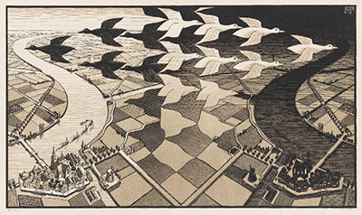
Maurits Cornelis (M.C.) Escher (1898-1972) is celebrated for his unique ability to represent the perfect fusion of mathematics and art, bringing these two seemingly disparate worlds together into a singular, cohesive vision. Born in the Netherlands, Escher began his professional life as a graphic artist specializing in woodcuts and lithographs, with no formal training in mathematics. His artistic direction was irrevocably shaped by a visit to the Alhambra palace in Spain, where he became captivated by the geometric decorations of the Moorish tiles. This experience became a defining moment, sparking a lifelong exploration of the mathematical concept of tessellation.

Tessellation: From Abstract Geometry to Fantastical Worlds

At the core of much of Escher’s work is tessellation, the mathematical principle of dividing a plane with regular, repeating patterns or "tiles" that fit together perfectly without overlapping or leaving gaps. While the concept is mathematically fundamental and deeply connected to the principles of symmetry, Escher’s genius lay in his ability to elevate this abstract idea. Instead of using simple geometric shapes, he infused his tessellations with a human and fantastical dimension. He populated his planes with intricate, interlocking figures of animals, lizards, draconic creatures, and goblins, transforming a Stark mathematical concept into a vibrant, imaginative world.

The Evolution of Escher’s Work: Two Distinct Periods

Escher's artistic career can be broadly categorized into two distinct periods. His early work was largely intuitive, driven by his personal fascination with repeating patterns and tessellations without direct collaboration with mathematicians. However, his work entered a new phase of profound depth and sophistication after he began to engage with the mathematical community. In this later period, his art delved into much more complex and abstract concepts. He explored themes of dimension, the topology (or shape) of space, and the nature of infinity. His artistic inquiries were so forward-thinking that some of his work has been seen as anticipating advanced scientific ideas; modern cosmologists have even theorized that the shape of our universe might be "Escher-shaped," suggesting his art touched upon deep features of modern cosmology.

Exploring Infinity, Paradox, and Perception

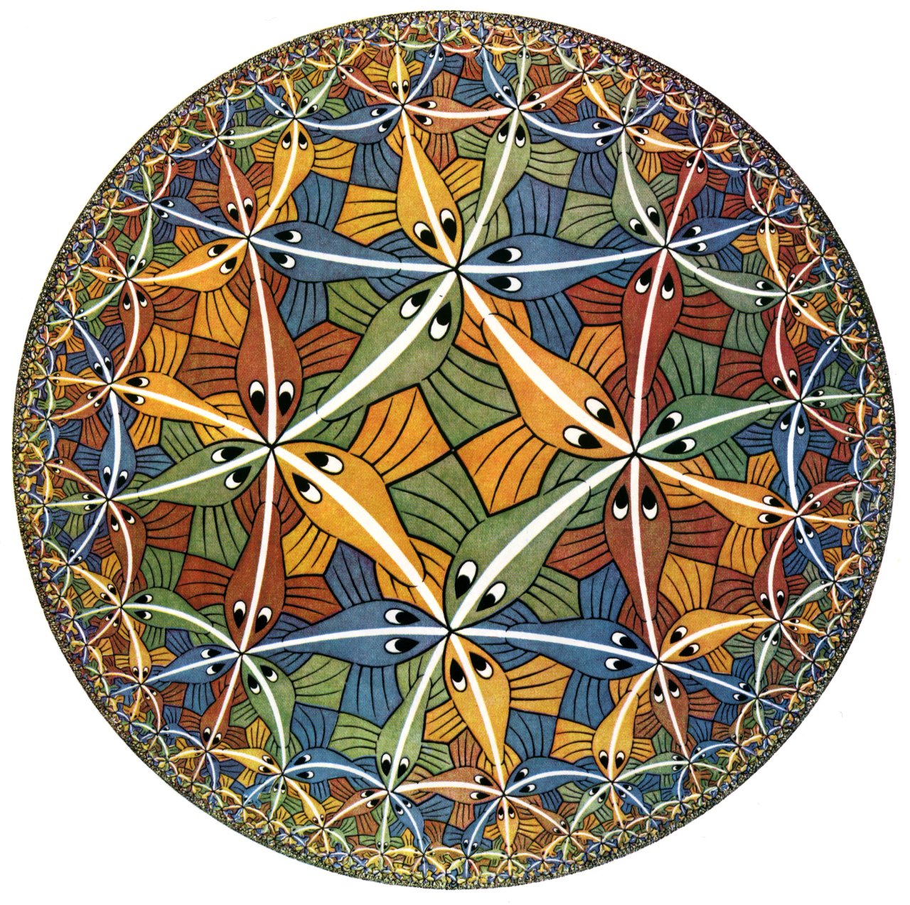
In his later period, Escher created some of his most famous and mathematically rigorous pieces. Using only basic drawing tools, he produced Circle Limit III, an astonishingly accurate representation of space as it edges towards infinity. The work’s precision was so remarkable that, nearly 40 years after its creation, mathematicians confirmed it was mathematically correct down to the millimeter.

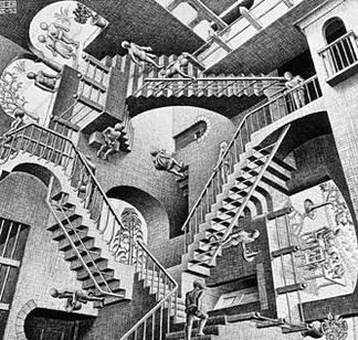
Escher was also deeply inspired by paradoxes and visual illusions. He was fascinated by the work of mathematicians like Roger Penrose, who created the "impossible triangle" and by the peculiar properties of the Möbius strip, an object that appears to have only one side. He used these ideas to create iconic images that look convincing at first glance but defy logic upon closer inspection. These visual illusions serve as a powerful commentary on the nature of perception, demonstrating that our brains do not passively see the world but actively interpret sensory input and make assumptions. Escher's work gives this interpretive part of the brain a "real workout," challenging our understanding of what is real and what is possible.

An Enduring Legacy in Mathematics and Art

Until his death in 1972, Escher remained intrigued by the concepts of infinity, reflection, and perception. His legacy endures, particularly within the world of mathematics. His prints are ubiquitous in university mathematics departments, adorning walls and appearing in textbooks. This is because his art speaks directly to mathematicians, offering a tangible, visual representation of the abstract beauty they find in their field. From a modern perspective, mathematicians understand more clearly what Escher was trying to achieve and can now even write down the formulas that describe the mathematical ideas behind his intuitive creations. Ultimately, M.C. Escher’s greatest contribution was his ability to bridge the gap between two cultures, using his artistic skill to show the wider world that the subject of mathematics is, in its essence, beautiful.

Most popular Esher work

M.C. Escher

Animation vs Math

Animation vs Geometry

Animation vs Physics

Animation cs Coding

the quantum Bayes' rule is defined as the rule for updating quantum states using the principle of minimum change (maximizing fidelity), and is mathematically realized by the Petz recovery map in many situations

The Kepler Problem